Viewing a Distribution Summary

If you have saved Final Values for an output, you can display a Distribution Result by right-clicking on the output (in a browser An alternative view of a GoldSim model, in which elements are displayed in a tree, and organized either hierarchically, or by type. or the output interface), or the element (if the output is the element's primary output For an element with multiple outputs, the output that has the same name as the element.) and selecting Distribution Result... from the context menu. By default, a Distribution Summary will be displayed.

If you are viewing a different type of display (either a chart or table), you can view a Distribution Summary by pressing the Chart or Table button at the top of the display (i.e., making sure both are buttons are cleared).

Note: When viewing a Distribution Result element A Result element that provides a way to view the final values of probabilistic outputs., the element "remembers"the last type of view that was displayed, and displays that view when you double-click on it.

The Distribution Summary view of a distribution result is similar in appearance to the dialog used for defining a Stochastic element An element that can be used to quantitatively represent the uncertainty in a model input..

A Distribution Summary looks like this:

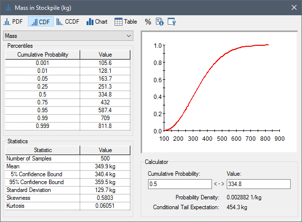
The preview pane (in the upper right-hand corner of the screen) shows a preview of the chart view of the distribution. You can copy the preview pane to the clipboard using Ctrl+C.

The left side of the screen displays a common set of percentiles for the distribution (in terms of Cumulative Probability/Value pairs).

The statistics for the distribution (Mean, 5% and 95% Confidence Bounds on the Mean, Standard Deviation The square root of the variance of a distribution. The variance is the second moment of the distribution and reflects the amount of spread or dispersion in the distribution., Skewness A measure of the symmetry of a distribution. A symmetric distribution has a skewness of 0. The skewness is a function of the third moment of the distribution., and Kurtosis A measure of how "fat" a distribution is relative to a normal distribution with the same standard deviation. A normal distribution has a kurtosis of 0. The kurtosis is a function of the fourth moment of the distribution.) are shown directly below the distribution's percentiles. The significance of these statistics is described in Appendix A of the GoldSim User’s Guide. The number of realizations (Number of Samples) is also indicated.

The Calculator section of the window allows you to compute the value associated with a particular percentile or the percentile associated with a particular value:

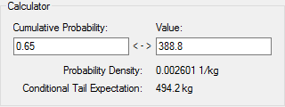
The Calculator also displays the Probability Density and the Conditional Tail Expectation The expected value of the output given that it lies above a specified quantile. That is, it represents the mean of the worst 100(1 - alpha)% of outcomes, where alpha is the specified quantile. for the specified Cumulative Probability/Value pair. The Conditional Tail Expectation is the expected value of the output given that it lies above a specified Cumulative Probability. That is, it represents the mean of the worst 100(1 - α)% of outcomes, where α is the specified Cumulative Probability.

Note: Calculation of the Conditional Tail Expectation is discussed in detail in Appendix B of the GoldSim User’s Guide.

The Distribution Summary has a variety of buttons at the top of the window:

The functions of these buttons are as follows:

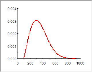
Display PDF: This displays the preview pane as a probability density function (PDF Probability Density Function. A function whose Y-axis can be interpreted as providing the relative likelihood that the value of a random variable would be equal to value specified on the X-axis. Hence, the dimensions of the Y-axis are the inverse of those of the X-axis (i.e., the probability per unit length of the X-axis).):

Note: The algorithm used to create a PDF plot is discussed in detail in Appendix B of the GoldSim User’s Guide. .

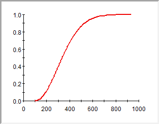
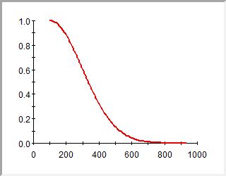
Display CDF: This displays the preview pane as a cumulative distribution function (CDF Cumulative Distribution Function. The integral of a probability density function.):

Display CCDF: This displays the preview pane as a complementary cumulative distribution function The integral of a probability density function. (CCDF Complementary Cumulative Distribution Function. The complement of the cumulative distribution function (which is the The integral of a probability density function).):

Show Chart: Selecting this button switches to a Chart view of the result. You can also toggle between the Distribution Summary View and the Chart View by double-clicking in the preview pane. Note that when viewing a Distribution Summary, both the Display Chart and the Display Table buttons appear deselected.

Show Table: Selecting this button switches to a Table view of the result. Note that when viewing a Distribution Summary, both the Display Chart and the Display Table buttons appear deselected.

Show Confidence Bounds: If you press this button or press Ctrl+Shift+B, GoldSim will display confidence bounds on CDFs and CCDFs (they cannot be shown for PDFs):

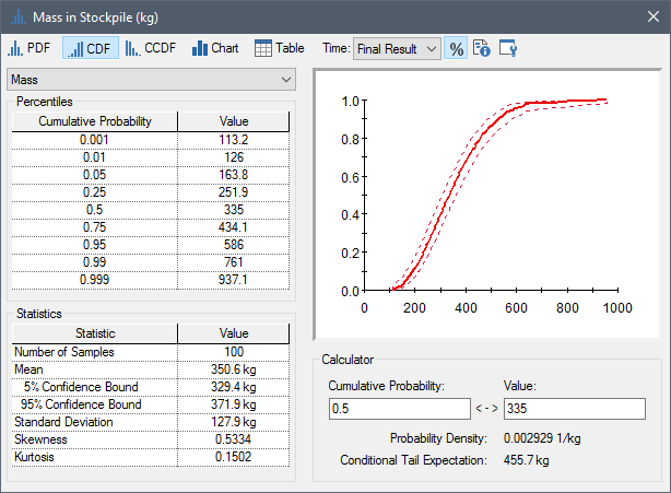
These bounds reflect uncertainty in the probability distribution due to the finite number of Monte Carlo realizations (as the number of realizations is increased, the uncertainty in the distribution decreases). The confidence bounds represent the 5% and 95% confidence limits on the distribution. The calculation of confidence bounds is discussed in detail in Appendix B of the GoldSim User’s Guide. Note that confidence bounds cannot be displayed if importance sampling An algorithm that biases sampling of probability distributions in order to better resolve the tails of the distributions. has been used in the model.

Show Result Array: Pressing this button displays a new (modal) window containing the result array. The result array represents a sorted table of all of the results, and is used to produce the charts and statistics for the distribution. The table shows the value, the weight, the number of occurrences of the value, the cumulative probability of the value, and the 5% and 95% confidence bounds for the value at that cumulative probability. (Note, however, that confidence bounds cannot be computed if importance sampling has been used in the model.)

Edit Properties: This provides access to the Result properties.

Note: If you press the Copy button (or Ctrl+C) from the Summary View of a Distribution result, the preview pane chart is copied to the clipboard.

By default, Distribution results operate on Final Values. That is, the display uses the values at the end of each realization A single model run within a Monte Carlo simulation. It represents one possible path the system could follow through time.. However, by defining Capture Times User-defined points in time during a simulation at which “Final Value” results are captured for result display. The final time point in the simulation is always included as a Capture Time, but additional times can be added., you can display results at any specified time. If you have created Capture Times, an additional drop-list is added to the display window to allow you to select the set of data (i.e., the results at the specified Capture Time) that you would like to display.

Note: When viewing distribution results produced by a nested Monte Carlo simulation A method for propagating (translating) uncertainties in model inputs into uncertainties in model results. (using a SubModel A specialized element that allows you embed one complete GoldSim model within another GoldSim model. This facilitates, among other things, probabilistic optimization, explicit separation of uncertainty from variability, and manipulation of Monte Carlo statistics.), the Distribution Summary dialog is modified somewhat and provides slightly different options.