Step 9: Editing Failure Modes and Adding Automatic Repair

Let's add some additional detail to the Component's beehive by adding failure modes and repair.

By default, the Function element allows you to specify a simple exponential failure mode that is not repaired. However, in many cases, the component's behavior cannot be accurately modeled in such a simple way. Moreover, many high value systems do not "fail" permanently - they are repaired and returned to service.

To demonstrate this capability, let's return to Edit Mode The state of a model when it is being edited and does not contain simulation results. (F4) and edit the failure modes for the Component. To do so, double-click on the Component element and clear the Use simple failure rate instead of advanced failure modes checkbox in the element's property dialog:

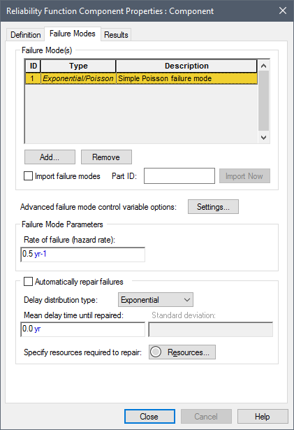
You'll notice that a new tab, called Failure Modes will appear. If you click on this tab you'll see the following dialog:

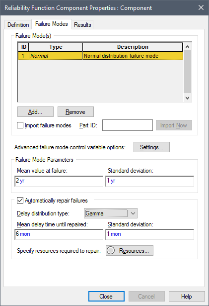
You'll notice that the initial exponential failure mode has been transferred over automatically by GoldSim. Let's delete this failure mode (press the Remove button), and add a Normal failure mode (by pressing the Add button and selecting "Normal"). Specify a mean of 2 yr and a standard deviation The square root of the variance of a distribution. The variance is the second moment of the distribution and reflects the amount of spread or dispersion in the distribution. of 1 yr.

You'll also notice that there is an Automatically repair failures option. Check that option, and specify a repair with a Gamma delay distribution, a mean time to repair of 6 months and a standard deviation of one month (month is abbreviated as "mon" in GoldSim). The dialog should then look like this:

If we wanted to, we could add additional failure modes. For the sake of simplicity, however, we'll stick with one for now. Press Close to close this dialog.

Delete the Milestone element An event element that records the time that an event occurs. (as it will generate warnings since it will now be triggered multiple times each realization A single model run within a Monte Carlo simulation. It represents one possible path the system could follow through time. due to the repair of the failure mode), and re-run the model (F5).

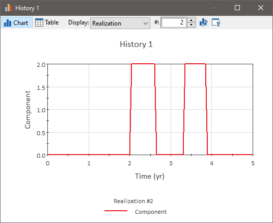
Let's view a time history plot of the status of the Component by double-clicking on the Time History Result element A Result element that shows the history of a particular output as a function of time.. From the Display drop-list at the top of the chart, select "Realization". This shows one realization at a time. You can toggle through realizations using the Realization spin control at the top of the window.

A typical result should look something like this:

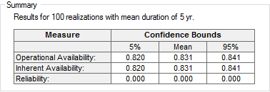
As can be seen, whenever the Component fails, it is repaired about 6 months later. If we look at the Results tab for the Component, we will see that the Availability The probability that a component or system is performing its required function at any given time. is relatively high (due to the repairs):