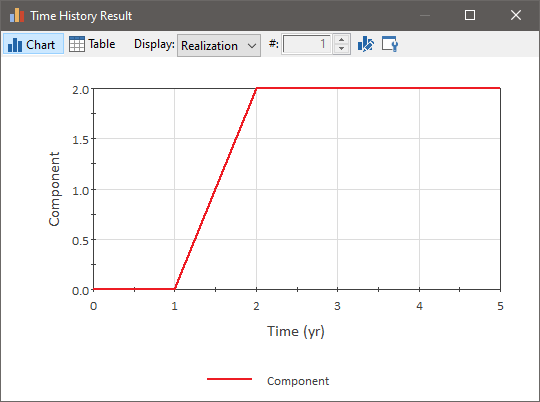
We can now run the model by pressing F5. After the simulation completes, right-click on the Function element and then left-click on Time History Result... in the context menu to view a time history plot of the result:

Note: Your result plot may look different, since this represents one random realization A single model run within a Monte Carlo simulation. It represents one possible path the system could follow through time. of the system.
What are we looking at here? This is actually the status of the Component over the course of the simulation. 0 indicates that the component is operating, and 2 indicates that the component has failed due to unmet Internal Requirements (in this case, the occurrence of the Simple Poisson failure mode).
Before thinking about this result plot further, it's important to first discuss how GoldSim moves the simulation through time. GoldSim "updates" the model as follows:
- The model is updated (all the elements in the model are recalculated) at the timesteps specified by the user. In this case, this means that element values are recalculated at 0 years, 1 year, 2 years, 3 years, 4 years and 5 years (as we have five timesteps). Values for time history plots are recorded at these user specified timesteps.
- GoldSim also updates the model upon the occurrence of certain kinds of "events". The failure of a reliability element is such an event. Hence, in this case, if the Component failed at 1.57 years, GoldSim would insert a new timestep A discrete interval of time used in dynamic simulations. at this point and update the model.
Note, however, that although the elements in the model are updated when such an event occurred, values for time history plots are only recorded at the user specified timesteps (in this case, 0, 1, 2, 3 ,4 and 5 years).
Given this information, we now know that the result shown above indicates that in this particular random realization (again, yours may be different), the Component failed sometime between 1 and 2 years. In the next step, we will determine exactly when the Component failed.
- Step 1: Creating a Dynamic Reliability Model
- Step 10: Adding Hierarchy (Sub-Components) to a Reliability Model
- Step 2: Adding a Reliability Function Element
- Step 3: Running the Model and Viewing a Simple Result
- Step 4: Determining the Time of Failure Using a Milestone Element
- Step 5: Increasing the Level of Time Discretization
- Step 6: Computing Reliability and Availability
- Step 7: Running Multiple Realizations of a Reliability Model
- Step 8: Viewing Monte Carlo Results for a Reliability Model
- Step 9: Editing Failure Modes and Adding Automatic Repair
- Where Do I Go From Here?