Step 5: Increasing the Level of Time Discretization

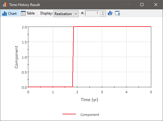
Let's add some additional timesteps and rerun the model to see how the time history plot changes.

To do this, you'll need to return to Edit Mode The state of a model when it is being edited and does not contain simulation results. by pressing F4. Then, open the Simulation Settings dialog (by pressing F2) and change the Basic Step length to 0.05 yr.

We can now close the Simulation Settings dialog and rerun the model (F5).

If you mouse over the Milestone element An event element that records the time that an event occurs., you will notice that the time of its occurrence hasn't changed from when you looked at them the last time your ran the model (since by default, random numbers generated to produce the events are repeatable).

However, the time history plot will change significantly. We can see this by right-clicking on the Function element and then left-clicking on Time History Result... in the context menu to view a time history plot of the result:

Notice how the change in the component's status from 0 to 2 is now seen to indeed occur around 1.85 years due to the additional timesteps.

Note: As pointed out previously, your result plot will be different, since this represents one random realization A single model run within a Monte Carlo simulation. It represents one possible path the system could follow through time. of the system.