In some situations, the behavior of a component (with regard to failure) may change significantly over time. There are two ways to model this type of behavior:
- The parameters of the failure mode can be specified to change over the course of the simulation (i.e., you can vary distribution parameters dynamically); or
- You can choose to model a component's behavior using multiple independent failure modes.
An example of this type of situation can be found in electronic components. These components typically have a high rate of failure initially (often called a burn-in period), and then a very low rate of failure for a period of time before the failure rate begins to rise again (producing a bathtub shaped failure distribution).
GoldSim does not have a "bathtub shaped distribution" that you can select from the failure mode list. Instead, to model this, we could set up an exponential distribution where the failure rate is a function of the elapsed time of the simulation (initially, the failure rate would be high, then drop to near zero, and increase again at the end of the component's lifespan). Alternatively, we could combine two or more independent failure modes to produce the same sort of behavior.
If we use multiple failure modes, we can make use of a special failure mode, called Defective Component. This failure mode is specifically designed for modeling the burn-in period. It only affects a proportion of components, and if a component is affected, the component fails according to an exponential distribution with a failure rate you specify. Components that are not affected by the Defective Component mode fail according to the remaining failure modes that you've specified, and components that are affected can still fail as a result of any other failure modes you might specify.
The model file BurnInPeriod.gsm, found in the Reliability Examples folder in your GoldSim directory (accessed by selecting File | Open Example... from the main menu), illustrates this second approach.
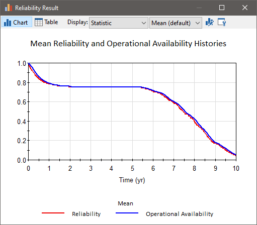
In this file, there is a single function element with two failure modes.The first is a Defective Component failure mode, affecting 25% of components, with a failure rate of 2 yr-1. This failure mode represents the failures during the burn-in period. The second failure mode is a normal failure mode with a mean value at failure of 8 years and a standard deviation of 1.3 years, representing end-of-life failures.
When you run the model and view plots of the Mean Reliability and Availability The probability that a component or system is performing its required function at any given time., you will notice the following:
- The Mean Reliability and Availability time histories are identical. This is because the failures are not repaired, and hence availability and reliability time histories measure the same thing. (There will be minor differences in the plots because Reliability is computed instantaneously, while Availability is computed based on averaging over a small time period previous to the time point.)
- You'll see that there is an exponential drop in those metrics almost immediately down to about 75% (the effect of the Defective Component failure mode). After that, the availability and reliability plateau, until failures begin to occur as a result of the Normal failure mode that has been specified.

- Example: Creating User-Defined Base Variables
- Example: Handling Actions Internally
- Example: Modeling Changing Operational Environments Using Failure Mode Acceleration
- Example: Modeling Component Maintenance and Replacement
- Example: Modeling Dependencies on Other Reliability Components
- Example: Modeling Dynamic Failure Mode Behavior Such as Burn-In
- Example: Modeling Non-Fatal Failure Modes
- Example: Modeling Resource Requirements for Reliability Elements
- Example: Modeling the Switchover to a Backup Component
- Example: Understanding the Differences Between Failure Mode Base Variables
- Example: Using Custom Reliability Outputs to Report Throughput Calculations
- Example: Using Reliability Elements for a Dam Risk Assessment
- Example: Using Reliability Elements to Model Failing Pumps
- Example: Using the Reliability Element's Primary Output
- Example: Working with Internal and External Requirements