GoldSim provides an advanced feature for dynamically revising distributions during a simulation using "simulated Bayesian updating". This feature is most valuable when using GoldSim to simulate a project of some kind (e.g., developing a new product, building a new facility). It is often the case that as a project progresses, additional information about uncertain variables is acquired. From the project operator's point of view, their uncertainty is decreasing, and hence as time progresses, the probability distributions used in their model of the project are converging towards the true values of the variables. As their knowledge increases they are better able to make appropriate decisions for the project's path forward.
When simulating a project in this manner using GoldSim, the model that is constructed will use Stochastic elements to specify the initial probability distributions of uncertain parameters, and a Monte Carlo sampling process will be used to pick the “true” values of those parameters. Given that starting point, simulated Bayesian updating can be used to simulate the additional information that will accrue as the project progresses. This in turn can be used to simulate the decisions that would be made based on the new information.
To support this, GoldSim allows you to define an "uncertainty reduction factor" for an uncertain variable. To do so, you must create a new Stochastic and specify its distribution type as an "Externally-defined Distribution":
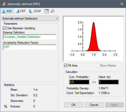
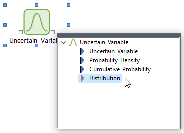
The uncertain variable (whose uncertainty is being reduced as the model progresses) is entered in the External Definition field for this new Stochastic. This must be a link to the Distribution output of a Stochastic element An element that can be used to quantitatively represent the uncertainty in a model input.. The Distribution output is a complex output that contains all the information regarding the distribution. It is the fourth output of a Stochastic:
You must then check the Use Bayesian Updating checkbox, and then enter a value for the Uncertainty Reduction Factor. This dimensionless factor, which must be between 0 and 1, approximates the extent to which the original distribution's standard deviation The square root of the variance of a distribution. The variance is the second moment of the distribution and reflects the amount of spread or dispersion in the distribution. has been reduced at any point in time. Essentially, this allows you to define how the initial uncertainty about the original distribution is reduced. As such, the Uncertainty Reduction Factor will almost always have an initial value of 1 (no reduction of uncertainty), and become smaller as a function of time (typically by changing in discrete steps representing points in time when new information has been obtained).
To understand the mechanics of how simulated Bayesian updating works, let us first examine a simple model that illustrates how the Externally-defined distribution is modified by a time-variable Uncertainty Reduction Factor. Subsequently, we will describe a (simplistic) real-world application.
The example model described here can be found in the file BayesianUpdating.gsm in the General Examples/Stochastic folder of your GoldSim directory (accessed by selecting File | Open Example... from the main menu). It is recommended that your open that file and follow along during the discussion below.
In a Container An element that acts like a "box" or a "folder" into which other elements can be placed. It can be used to create hierarchical models. named "Basic_Concepts", you will see a very simple model that looks like this:
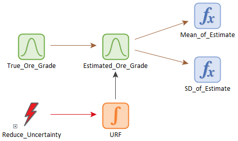
The True_Ore_Grade represents the variable that is being studied (and whose uncertainty is being reduced during the simulated project). In this example, it is a Normal distribution with a mean of 10 and a standard deviation of 3. The Estimated_Ore_Grade represents the updated distribution resulting from studies carried out on the ore grade during the project. It is an External Distribution whose primary input is the True_Ore_Grade, and whose Uncertainty Reduction Factor is defined by the variable URF:
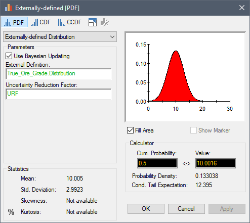
URF is simply an Integrator with an initial value of 1 (no uncertainty reduction) that is updated by a Discrete Change at discrete points in time (representing studies that have reduced the uncertainty in the ore grade). In this example, URF is simply reduced by a factor of 0.2 every 10 days for a period of 50 days:
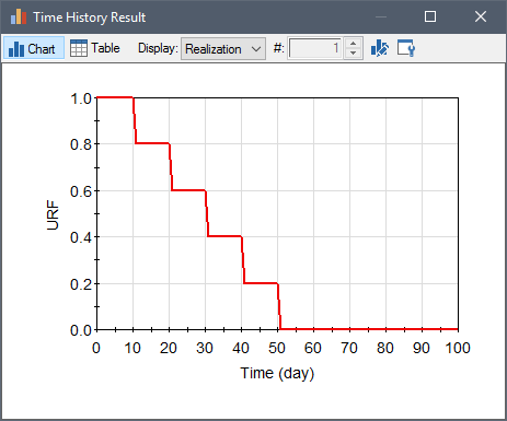
Hence, after 5 days, the uncertainty in the ore grade has actually been reduced to zero (i.e., it is assumed that the ore grade is perfectly known at 50 days).
Given this information, it is instructive to view how the Estimated_Ore_Grade distribution changes as a function of time. Although we can't easily view the distribution in the middle of a simulation, we can examine its statistics and see how they change with time. To do so, we take advantage of two of GoldSim's built-in functions: PDF Probability Density Function. A function whose Y-axis can be interpreted as providing the relative likelihood that the value of a random variable would be equal to value specified on the X-axis. Hence, the dimensions of the Y-axis are the inverse of those of the X-axis (i.e., the probability per unit length of the X-axis)._Mean and PDF_SD, which return the mean and standard deviation, respectively, of a specified distribution.
The plot below shows how the mean and the standard deviation of the Estimated_Ore_Grade distribution change with time. The plot also includes the True_Ore_Grade:
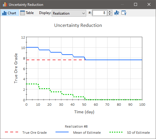
Every realization A single model run within a Monte Carlo simulation. It represents one possible path the system could follow through time. of the model produces a different sampled True_Ore_Grade. In this particular realization, the True_Ore_Grade was sampled to be just less than 8. As can be seen, the initial mean and standard deviation of the Estimated_Ore_Grade are 10 and 3, respectively (the same as the statistics for the True_Ore_Grade distribution). However, starting at 10 days, more information is learned about the ore grade. This has two effects on the Estimated_Ore_Grade distribution: 1) the standard deviation is reduced; and 2) the mean approaches the true value. Whenever new information is obtained (in this example, every 10 days), the standard deviation is further reduced, and the mean moves closer to the true value. At 50 days (when it is assumed that "perfect information" is obtained), the standard deviation goes to zero, and the mean converges to the true value.
Now that we have explained conceptually how simulated Bayesian updating is carried out, let's now expand on this example slightly to illustrate how it might actually be used in a real model. The example model described here can be found in the same file (BayesianUpdating.gsm) in the General Examples/Stochastic folder of your GoldSim directory (accessed by selecting File | Open Example... from the main menu). It is in a Container named "Example_Application".
The example considers the case of a proposed new mine. Initially the mean ore grade may have considerable uncertainty, but as successive studies are carried out, additional information is obtained and the uncertainty about the mean ore grade is reduced. Let's further assume that once you have a particular level of certainty regarding the value, you will act in one way or another.
We will represent this by starting with the previous example, and making one change and one addition:
- We will assume that only four studies are carried out (at 10, 20, 30 and 40 days), each reducing the Uncertainty Reduction Factor by 0.2, such that (as would be realistic) perfect information regarding the ore grade is never obtained.
- We will assume that the estimated ore grade must be greater than 12 for the project to proceed. Because the ore grade cannot be known with certainty, however, this decision must be based on probabilities. In particular, when simulating the project, it is assumed that the project will proceed if and only if we have at least 50% confidence that the ore grade is greater than 12 (i.e., we will proceed if the probability of the ore grade being at least 12 exceeds 50%).
The probability of the ore grade being at least 12 is another statistic (that is changing with time as more information is obtained) that can be computed using one of GoldSim's built-in functions (PDF_CumProb). The plot below shows how the probability of the ore grade being at least 12 changes with time for a particular realization:
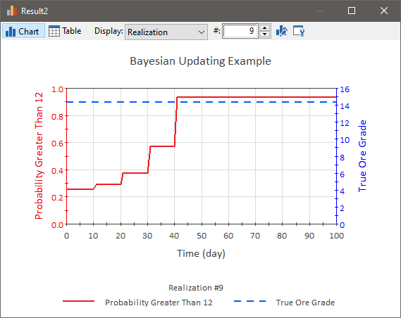
In this realization, the true value is sampled to be approximately 14.3. Given the original distribution (Normal distribution with mean 10 and standard deviation 3), the original probability of the value being greater than 12 is about 25%. As the uncertainty in the ore grade is reduced, the probability of the ore grade being greater than 12 increases, until at 30 days, it jumps above 50% to 57% (and at 40 days jumps to 93%), and hence the project can proceed.
In this simplified model, when this occurs, an event is triggered which in a real model could trigger the next phase to begin:

Although this example is simple, it illustrates how simulated Bayesian updating can be used to simulate additional information that is obtained as a project progresses, and how this can in turn be used to simulate the decisions that would be made based on the new information.
Learn more
- Applying Importance Sampling to a Stochastic Element
- Browser View of a Stochastic Element
- Controlling When a Stochastic Element is Sampled
- Correlating Stochastic Elements
- Creating a Stochastic Vector
- Customized Importance Sampling Using User-Defined Realization Weights
- Dynamically Revising Distributions Using Simulated Bayesian Updating
- Specialized Functions That Operate on Distributions
- Specifying a Deterministic Value for a Stochastic
- Specifying the Distribution for a Stochastic Element
- Stochastic Distribution Types
- Triggering a Stochastic