Mathematics of Simulated Bayesian Updating
The conventional approach to sampling an uncertain variable is to first sample a random value (from a uniform distribution between 0 and 1), and then use this value as input to the inverse cumulative distribution function for the uncertain variable.
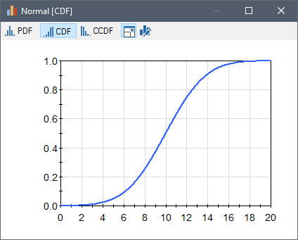
For example, the CDF Cumulative Distribution Function. The integral of a probability density function. for a Normal distribution (with mean 10 and standard deviation The square root of the variance of a distribution. The variance is the second moment of the distribution and reflects the amount of spread or dispersion in the distribution. 3) looks like this:

To sample this distribution, GoldSim would first sample a random value from a uniform distribution between 0 and 1 (such that all values were equally likely), and use this as the cumulative probability level for the sampled variable. It would then map that probability to a value. For example, if 0.4 was sampled from the uniform distribution, that would map to a value for the variable of approximately 9 in this case.
To understand how simulated Bayesian updating is carried out, recall that two separate Stochastic elements must be defined to carry it out: 1) a Stochastic representing the "true" value; and 2) a Stochastic (defined as an Externally-defined distribution with a specified Uncertainty Reduction Factor) representing the "updated" distribution. When doing Bayesian updating, the key point is that the random value on the probability axis for the "updated" distribution is not sampled from a uniform between 0 and 1; rather, it is sampled from a beta distribution, whose shape depends on the sampled "true" value and the specified Uncertainty Reduction Factor for the "updated" distribution.
The specific way this is done is as follows:
-
A random number is selected in order to sample the distribution representing the "true" value.
-
In order to sample the "updated" distribution, a beta distribution is created on the probability axis for the distribution. This beta distribution has a minimum value 0 and maximum value 1. Its standard deviation is calculated as the product of the default standard deviation value for sampling the probability axis (0.288675, for a uniform distribution) and the Uncertainty Reduction Factor. The mean of the beta moves linearly from the original mean (0.5 for a uniform distribution) towards the sampled probability level for the original Stochastic as the Uncertainty Reduction Factor ranges from 1 to 0.
Hence, if we assume that the sampled random number for the "true" value is 0.3, and the Uncertainty Reduction Factor is 0.5, then the beta distribution that is created would have a mean of 0.4 (half way between 0.5 and the sampled value 0.3) and a standard deviation of 0.288675*0.5. -
This beta distribution is then sampled (returning a value between 0 and 1).
-
This value is then used as input to the inverse cumulative distribution function The integral of a probability density function. for the original Stochastic.
Note that as the Uncertainty Reduction Factor approaches 0, the "updated" value approaches the "true" value.
The approach described above is used for all continuous distributions. As described above, it effectively increases the likelihoods of "updated" values closer to the "true" result, and reduces the likelihoods of values that are further away from it. This is usually an appropriate approach, as most tests of continuous variables will have a limited accuracy and resolution, and as such, the probabilities of nearby values are correlated. However, for a discrete distribution (e.g., “is it an apple, an orange, or a pear?”) there is likely no correlation between the probabilities of nearby values (and for Boolean, the concept of "nearby" values does not even apply). Accordingly, a different approach (described below) is used for Boolean and Discrete distribution types. However, the approach described above for continuous distributions is also used for the results of binomial, Poisson, and other discrete-valued distributions, as there typically would be a correlation between nearby values for these distributions.
For the Boolean and the Discrete distributions the uncertainty reduction works differently. In these cases, for the "updated" distribution, the probability of the "true" value is increased linearly from its original probability level to a value of 1 as the Uncertainty Reduction Factor drops from 1 to 0. For all other outcomes, the original probabilities are simply multiplied by the Uncertainty Reduction Factor, dropping to 0 as the Factor approaches 0. As was the case for the continuous distributions, sampling is accomplished via an auxiliary probability distribution A mathematical representation of the relative likelihood of a variable having certain specific values. It can be expressed as a PDF (or a PMF for discrete variables), CDF or CCDF. that modifies the sampled probability levels, but instead of a beta distribution, a cumulative distribution is used in order to have the desired effect.