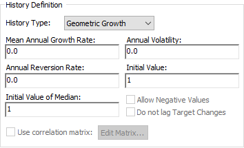
Selecting "Geometric Growth" for the History Type field of a History Generator An element that generates stochastic time histories of variables. A stochastic time history is a random time history that is generated according to a specified set of statistics. element allows you to define a history that grows geometrically with time. This means that the rate of growth and the amount of volatility are proportional to the current value. Among other things, this type of history is appropriate for variables such as security prices.

In its simplest form, this type of history requires three
inputs (Mean Annual Growth Rate,
Annual Volatility, and Initial Value). The other two inputs
(Annual Reversion Rate and Initial Value of Median) are only required if you wish the history to
revert toward its median (and this is discussed in
the next
Mean Annual Growth Rate. This is the mean annual logarithmic growth rate (μ'), where Vi is the value at time i:
Although this is a rate (i.e., time-based), because it is "hard-wired" to be an annual value, this input is dimensionless. That is, it represents the logarithmic growth rate over a year. It can be positive, negative, or zero.
If the logarithmic growth rate is measured over a different time period (e.g., monthly), this can be scaled by direct multiplication. For example a mean monthly logarithmic growth rate can be converted to a mean annual logarithmic growth rate by multiplying it by 12.
Annual Volatility. This is the standard deviation The square root of the variance of a distribution. The variance is the second moment of the distribution and reflects the amount of spread or dispersion in the distribution. of the annual logarithmic growth rate (σ'):
This is a dimensionless value that must be non-negative.
Note: As pointed out above, the volatility for a geometric growth history is, by definition, dimensionless. This is different than the volatility for a random walk history, which has dimensions An output attribute for an element that defines the dimensionality (in terms of Length, Time and other fundamental dimensions) of the output..
If the logarithmic volatility is measured over a different time period (e.g., monthly), and the rate of reversion to the median The 50th percentile of a distribution. is zero, this can be scaled by the square root of the time period. For example, a mean monthly logarithmic volatility can be converted to a mean annual logarithmic volatility by multiplying it by √12.
Initial Value. This is the initial value of the time history (the value at time zero). It has the same dimensions as the output. It must be a positive number.
If the Annual Reversion Rate is set to zero (the default), GoldSim generates successive values as follows:
where Vnew is the new value, Vold is the previous value, Δt is the time between the two values, ε is a random standard normal value (sampled from a distribution with mean 0 and standard deviation 1), and μ' and σ' are as defined above.
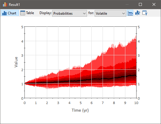
For constant values of the Mean Annual Growth Rate and Mean Annual Volatility, this results in a history that (on average) grows exponentially, and whose standard deviation of the logs increases as the square root of time:

At any given time, the distribution of values is log-normal.
The logarithmic input definitions for the Growth Rate and Volatility, as used by GoldSim, are those typically used by academic financial analysts. However, it may be difficult to find data expressed using these formal definitions. Some simple approaches for converting available data to these forms are as follows:
Converting from Geometric Mean Returns
Typically, the performance of individual securities is reported as "average annual total returns". Mathematically, this actually represents the geometric mean of the annual returns over a period:
You can use GoldSim's built in gm2cm function to convert a geometric mean annual return to an arithmetic mean log annual return.
If the standard deviation of the average annual total returns is also available:
where
This can then be used (in conjunction with the geometric mean of the returns) to compute the volatility using GoldSim's geo2vol function.
Converting from Arithmetic Mean Returns
In some cases, you may have return rate statistics reported in terms of the arithmetic mean of the annual return over a period (μa, defined above).
You can use GoldSim's built in ari2cm function to convert an arithmetic mean annual return (and a standard deviation) to an arithmetic mean log annual return, and the ari2vol function to convert a standard deviation (and an arithmetic mean) of the annual return to the standard deviation of the log annual return (the volatility).