This example illustrates the use of a Time Series where the input data represent changes over specified intervals. This option is usually used to output cumulative values (e.g., cumulative rainfall, cumulative sales) and/or rates (e.g., sales rates, rainfall rates) that are specified by defining incremental changes in a variable (e.g., monthly sales, monthly rainfall) over specified intervals.
The example can be viewed in the file named BasicTimeSeries.gsm, which can be found in the TimeSeries subfolder of the General Examples folder in your GoldSim directory (accessed by selecting File | Open Example... from the main menu).
It is important to understand that when this option is selected, the Primary Output For an element with multiple outputs, the output that has the same name as the element. of the Time Series is not the specified time series itself. Rather, it is the cumulative value of the variable at each point in the simulation (assuming that the specified changes occur uniformly over each interval). This option therefore typically takes advantage of the Rate_of_Change output.
The Rate_of_Change output for a Time Series that is defined as a series of changes over specified intervals represents the rate of change of the cumulative value. For example, if the data was entered as monthly sales increments, the Rate_of_Change would represent the sales rate.
The rate is computed by dividing the incremental change in the variable over the interval by the interval length. GoldSim assumes that the variable (e.g., cumulative rainfall or sales) changes uniformly over the time period, which means that the rate of change is constant over the interval (i.e., it "stair-steps").
Note: This option is particularly useful for time series that are collected at variable time points (e.g., once per month, since the number of days in a month is not constant). GoldSim is able to readily turn such data into rates.
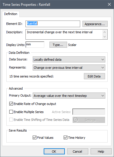
In this example, the input data represent the total rainfall over specified time periods:

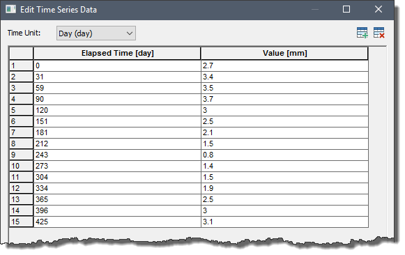
The actual data set looks like this:

In this example, between 59 and 90 days, the value is assumed to have changed by 3.5 mm.
Note: There are two options for representing time series that represent changes over specified intervals. You can specify that the data changes over the next interval (as specified above), or you can specify that the data changes over the previous interval. In the latter case, the data set shown above would imply that between 59 and 90 days, the value changed by 3.7 mm. (In order for the two representations to provide the same results, you would need to shift the data column by one row.)
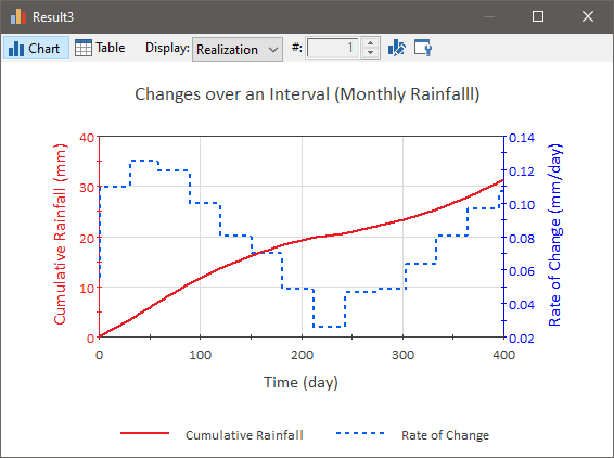
The Primary Output and the Rate_of_Change outputs for this particular example are shown below:

The Primary Output is computed by integrating the changes, assuming that the changes occur uniformly over each interval. Note that this implies that the rate of change is constant over the interval (i.e., it "stair-steps"). This is the appropriate way to represent variables that are measured on a monthly basis (e.g., sales, rainfall) and need to be converted into rates for use in your model (e.g., sales rate, rainfall rate).
Note: If the data is specified to represent a "Change over an interval" (either next or previous), then the first data point must be at or before the beginning of the simulation, and the last data point must be at or beyond the end of the simulation. That is, if you have specified time entries as elapsed times, the first data point must be less than or equal to zero, and the last data point must be greater than or equal to the simulation duration. If you have specified time entries as dates, the first date must be at or before the start time for the simulation, and the last date must be at or after the end time for the simulation.