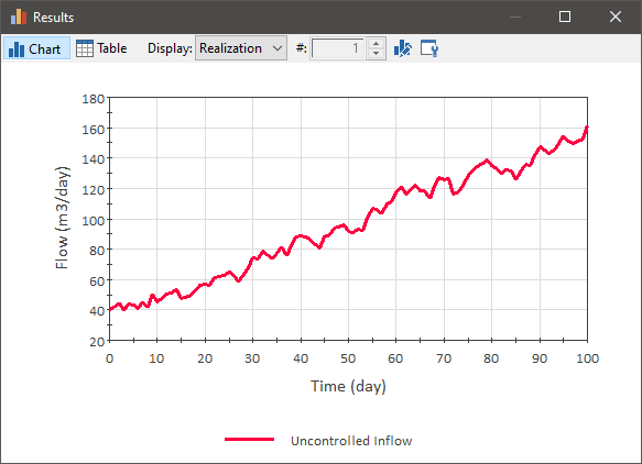
If the uncontrolled inflows and outflows to your process follow a trend or a pattern (e.g., a seasonal pattern), Proportional Controllers with a constant Bias and Gain would result in poor performance.
In order to successfully use a Proportional Controller in this case it is necessary to take the extra step of defining the Bias as being time variable in order for the Controller to perform well.
Recall that if you are simulating an Outflow Controller, the Bias can be thought of as the sum of the expected uncontrolled inflows minus other expected uncontrolled outflows. If you are simulating an Inflow Controller, the Bias can be thought of the sum of the expected uncontrolled outflows minus other expected uncontrolled inflows. So if the expected uncontrolled inflows and outflows are time variable (e.g., have a trend), it simply means that the Bias should represent this (and be specified as a function of time).
Consider an example in which we have an Outflow Controller (e.g., which adjusts a pumping rate out of a pond) and the pond has an uncontrolled inflow that is steadily increasing (and is noisy):

Conceptually, what we want to do here is actually monitor two items in order to adjust the outflow: the process variable and the uncontrolled inflow. That is, if you were manually trying to maintain the target value, you would want to consider two things in order to determine what the outflow should be: 1) how far is process variable from the target; and 2) how much inflow is expected going forward. For the second item, what you need is a forecast of the inflow. In a simulation model The implementation of a mathematical model of a system within a specific computational tool (or set of tools)., we can forecast future values based on observed values in the past. The simplest such forecast would be that the next value will be the same as the last value we observed. But, of course, there are other forecast methods as well. One of the most common (and simplest to implement) forecast method is exponential smoothing. In exponential smoothing, the forecast is based on an exponentially-weighted average of past observations. This can be readily simulated in GoldSim using an Information Delay A delay element that delays information signals, and does not enforce conservation of the signal. It is intended to be used to simulate delays in measuring, reporting, and/or responding to information..
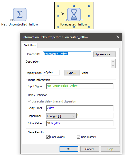
For this example, we can create a forecast of the inflow by inputting past values of the inflow into an Information Delay as follows:

The Input Signal is the net uncontrolled inflow (the sum of the uncontrolled inflows minus the sum of the uncontrolled outflows). (In this simple example, there are only uncontrolled inflows and there are no uncontrolled outflows; if there was, we would want the Input Signal to be the difference between uncontrolled inflows and uncontrolled outflows.) Setting the Erlang Dispersion to 1 results in the Information Delay outputting an exponentially smoothed forecast of the Input Signal. The Delay Time controls how heavily weighted previous values are. The larger the Delay Time, the more heavily weighted older values are (i.e., the farther the forecast reaches back in time to generate the forecasted value).
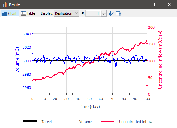
If we then use the Forecasted Inflow as the Bias for the Controller, we see that the Proportional Controller performs quite well:

This should not be surprising, as we are using more information to determine the output for the Controller (both the current value of the process variable, as well as previous values for the uncontrolled inflow).
The example model above which illustrates using a forecast to define the Bias for a Proportional Controller (ProportionalForecast.gsm) can be found in the General Examples/Controllers folder in your GoldSim directory (accessed by selecting File | Open Example... from the main menu).