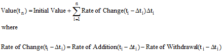
How a Reservoir Element Computes its Primary Output

Numerically, GoldSim approximates the integral represented by a Reservoir as a sum:

In these equations, ∆t_i is the timestep length just prior to time t_i (typically this will be constant in the simulation), and Value(t_n) is the value at end of timestep n. Note that the Value at time t_i is a function of the Rates of Addition and Withdrawal at previous timesteps (but is not a function of these Rates at time t_i).

Note that if you specify Upper or Lower Bounds for a Reservoir, the equation shown above is constrained by the specified bounds (i.e., the Value cannot exceed the Upper Bound and can not be less than the Lower Bound).

Reservoirs and Integrator elements use the same numerical integration method, referred to as Euler Integration. A simple example illustrating this integration method is provided in the topic discussing how an Integrator element computes its output.

The key assumption involved in this integration method is that at any point in time, the Rates of Change (Additions and Withdrawals) represent the rates over the next timestep, and those rates are assumed to be constant over the timestep. Euler Integration is discussed in additional detail in Appendix F of the GoldSim User’s Guide.

Note: Euler integration is the simplest and most common method for numerical integration. However, if the timestep is large, this method can lead to significant errors. This is particularly important for certain kinds of systems in which the error is cumulative (e.g., sustained oscillators such as a pendulum). In these cases, these errors can be reduced by using Containers with Internal Clocks, which allow you to locally use a much smaller timestep.