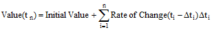
How an Integrator Element Computes its Output

Numerically, GoldSim approximates the integral represented by an Integrator as a sum:

where ∆t_i is the timestep length just prior to time t_i (typically this will be constant in the simulation), and Value(t_n) is the value at the end of timestep n. Note that the Value at a given time is a function of the Rate of Change at previous timesteps (but is not a function of the Rate of Change at the current time).

In order to better understand how GoldSim carries out this numerical integration, it is worthwhile to consider the following example. Consider a car that drives on a road for five minutes. We input the time history of the velocity of the car as follows:

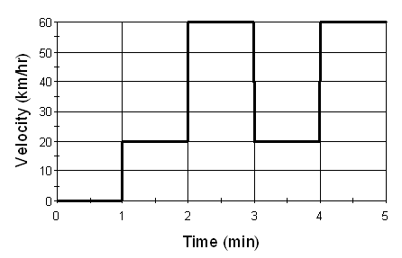
Hence, it is stopped for the first minute, travels at 20 km/hr for the second minute, 60 km/hr for the third minute, 20 km/hr for the fourth minute, and 60 km/hr for the fifth minute.

If we put this time history into an Integrator element, and run the simulation for 5 minutes with a constant 1 minute timestep, we get the following for the cumulative distance traveled (assuming an Initial Value of 0):

(This example model, named Integrator.gsm, can be found in the General Examples folder in your GoldSim directory, accessed by selecting File | Open Example... from the main menu.)

The manner in which GoldSim computed these results is summarized in the following table:

i timestep	t_i (min)	Velocity During Next Step Velocity(t_i)	Distance Traveled During Previous Step Velocity(t_i-∆t) * ∆t	Cumulative Distance Traveled at time = t_i
-	0	0 km/hr	-
1	1	20 km/hr	0 km/hr * 1 min = 0 km	0
2	2	60 km/hr	20 km/hr * 1 min = 0.333 km	0.333 km
3	3	20 km/hr	60 km/hr * 1 min = 1 km	1.333 km
4	4	60 km/hr	20 km/hr * 1 min = 0.333 km	1.666 km
5	5	-	60 km/hr * 1 min = 1 km	2.666 km

Note that the Value (cumulative distance traveled) at time t_i is independent of the Rate of Change (velocity) at time t_i. It is only a function of the Rates (velocities) at previous timesteps.

This particular numerical integration method is referred to as Euler integration, and is discussed further in Appendix F of the GoldSim User’s Guide. For the present purposes, it is sufficient to note that Euler integration assumes that the Rate of Change is constant over a timestep. Hence, if you specify that the Rate of Change to an Integrator varies linearly from 0 km/hr to 10 km/hr over 10 minutes, and simulate the system with a 1 minute timestep, GoldSim will approximate the velocity curve internally as a stair-step function:

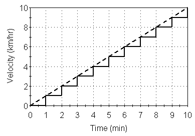
The dashed line represents the specified Rate of Change. The solid line illustrates how the Integrator element would interpret the Rate of Change, assuming a 1 minute timestep.

Note: By default, the Rate of Change at time t is treated as the constant rate of change over the next timestep (i.e., from t to t + Δt). GoldSim provides an advanced option to allow you to modify this behavior such that the Rate of Change at time t is treated as the constant rate of change over the previous timestep (i.e., from t to t - Δt).

Note: Euler integration is the simplest and most common method for numerical integration. However, if the timestep is large, this method can lead to significant errors. This is particularly important for certain kinds of systems in which the error is cumulative (e.g., sustained oscillators such as a pendulum). In these cases, these errors can be reduced by using Containers with Internal Clocks, which allow you to locally use a much smaller timestep.