This example shows how warranty costs for a product (e.g., a vehicle) can be computed based on a product sales rate and the expected warranty cost time history for a product using a Convolution element An element that solves a convolution integral..
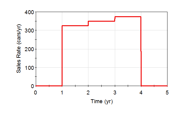
In this example, the input signal is the sales rate of the vehicle:

Sales will start one year in the future, and ramp slowly up for three years. The vehicle is only assumed to be produced for three years.
This can be entered into GoldSim as a Time Series.
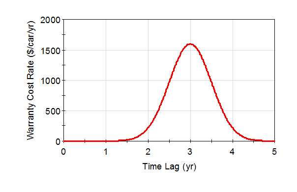
The Transfer function represents, on average, how warranty costs are expected to be incurred in the future (per vehicle):

This curve indicates that warranty costs start to be incurred about 1.5 years after the sale, reach a peak at 3 years after the sale, and no more costs can be expected to occur after about 4.5 years after the sale. Note that the units on the transfer function are $/car/yr (the curve integrates to 2000 $/car).
The output signal will then have dimensions An output attribute for an element that defines the dimensionality (in terms of Length, Time and other fundamental dimensions) of the output. of $/yr:
Output = Transfer Function * Input Signal * time
Output = $/car/yr * cars/yr * yr = $/yr
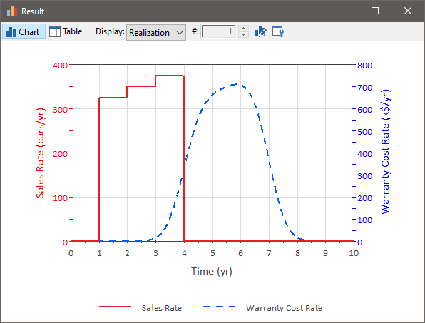
That is, the output represents the rate at which we can expect to incur warranty costs for all of the vehicles sold:

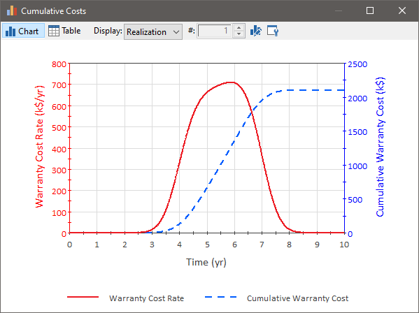
If we integrate the warranty cost rate (using an Integrator), we can compute the cumulative warranty costs:
