Failure distributions are frequency distributions in time. That is, they define the failure rate as a function of time. You define the shape of the distribution using one or more parameters (e.g., the uniform distribution requires a duration).
Note, however, that the parameters defining the container failure distributions cannot vary with time (i.e., a parameter that defines a distribution in time cannot vary with time). As a result, it is not possible for the failure rates to respond directly to time-varying conditions. That is, the failure distribution for a given mode must be defined assuming a given set of conditions. Any temporal changes in conditions (e.g., temperature, water saturation) that may affect the failure distribution must be known prior to its specification and indirectly incorporated into the form of the distribution.
The Effective Time, however, can be used to delay or modify failure distributions such that they can dynamically respond to time-varying conditions. For example, the failure rate could be specified to increase with increases in temperature or aggressive chemical conditions. The Effective Time represents the failure mode's view of how far along the time axis it is relative to the start-time of the defined failure distribution.
Hence, if the Effective Time increases faster than the elapsed time, this has the effect of accelerating failures (relative to that defined by the distribution); if the Effective Time increases at a slower rate than the elapsed time, this has the effect of decelerating failures. If the Effective Time temporarily does not increase at all as the elapsed time increases, this has the impact of temporarily stopping failures.
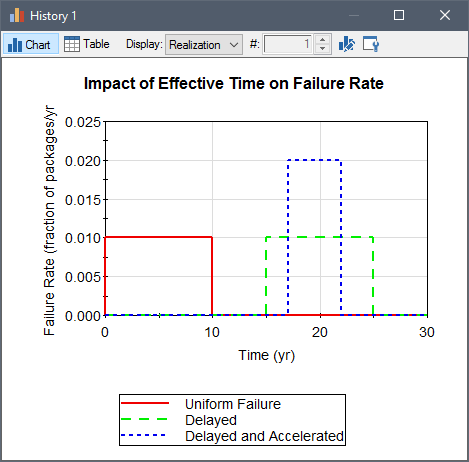
It is easiest to illustrate the use and physical significance of the Effective Time by considering an example. Suppose that we start with a failure distribution for a Source which is defined such that the packages fail uniformly over 10 years. Let's now consider two modifications to this distribution. In the first case, we wish to delay the start of failure by 15 years. In the second case, we wish to delay the start by 17 years, but once the distribution starts, we want the containers to fail at twice the rate. These three cases are illustrated graphically below:

Within GoldSim, we could achieve all three of these behaviors by defining a uniform failure distribution and specifying the Effective Time as follows:
| Case | Effective Time |
| uniform failure beginning immediately | Etime |
| uniform failure, start delayed by 15 years | Etime-15yrs |
| uniform failure, start delayed by 17 years, accelerated after start by factor of 2 | 2 * (Etime - 17yrs) |
Note that the default value for the Effective time is the elapsed time (Etime), which implies that the failure distribution starts at the beginning of the simulation and is not modified during the simulation in any way.
- Controlling the Outer Barrier Failure Algorithm
- Defining the Level of Containment
- Disrupting Packages Using Discrete Events
- Simulating Inner Barrier Failure
- Simulating Outer Barrier Failure
- Source Example #1: Barrier Failure and Solubility-Controlled Release
- Specifying Failure Distributions for Barriers
- Understanding Barrier Failure
- Using the Effective Time to Delay/Modify Failure Distributions