Example: Modeling Changing Operational Environments Using Failure Mode Acceleration

In many cases, a failure mode may be affected by multiple factors. For example, the wear on a turbofan engine may primarily be related to the number of hours it operates, but wear might be accelerated in hot environments. A failure mode’s acceleration features can be used to simulate the effects of different operational environments on the control variable by accelerating or decelerating the amount of wear for a given change in the control variable.

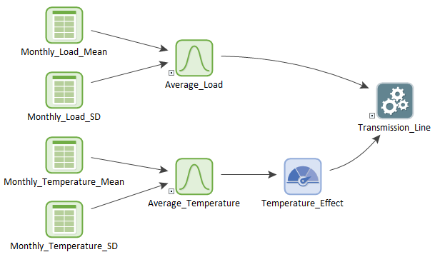
The model file Acceleration.gsm, found in the Reliability Examples folder in your GoldSim directory directory (accessed by selecting File | Open Example... from the main menu), is a simple model of a fictitious power transmission line. Its failure is time based, but it depends on the average monthly load on the system and the average monthly temperature. The line typically fails after 35 years (normally distributed with a standard deviation of 5 years) with an average load of 1MW, and mean operating temperatures between 0C and 20C.

Average loads that are lower (e.g., 500kW) induce lower wear (in this case, the line wears at 50% of the rate it would transmitting 1MW), while average loads that are higher cause higher wear (e.g., transmitting 2MW causes the line to wear twice as fast).

Temperature extremes also cause wear. Cold temperatures and the formation of ice increase wear below 0C (wear is multiplied by a factor of three), and high temperatures cause the lines to sag. As a result, every increase of 10C in the average temperature beyond 20C increases wear on the lines by a factor of 2.

Both the average load and average temperature are resampled each month, using month-by-month data for both values.

In the model, we have a reliability element representing the transmission line. It has a single, normal failure mode that is not repaired. If you view the Failure Modes tab, and click the Settings… button, you will see that an Acceleration Factor has been specified for this failure mode:

Temperature_Effect is a Selector element (a nested if statement) that is:

• 3 if the average temperature is below 0C;

• equal to the (Average_Monthly_Temperature – 20C)/10K * 2 if the average temperature is greater than 20C and

• 1 otherwise

In this way, we are able to combine the effects of time, load and temperature to get a more accurate picture of how the line would behave, even if it was not transmitting 1MW of energy at a temperature of between 0C and 20C.